On a suggestion from Michael, I have had a quick look at BON in a Box, which is a web-based biodiversity analysis platform using Docker containerised pipelines running R, Julia, and Python scripts.
It couldn’t be easier to get started. Install Docker and Docker Compose, and make sure you can access GitHub via SSH using a public key. [Run ssh-keygen -t ed25519 and then publish the resulting ~/.ssh/id_ed25519.pub to your GitHub account.]
apt install docker.io docker-compose-v2
Clone the GEO-BON’s repository and make a working copy of the runner.env file. This file can be edit to add API keys of datasets, but I don’t have any so the default file is fine.
git clone git@github.com:GEO-BON/bon-in-a-box-pipelines.git
cd bon-in-a-box
cp runner-sample.env runner.env
To start the server run ./server-up.sh. There is also ./server-down.sh to stop the server.
The first run downloads the required Docker containers so takes a few minutes. Once complete visit http://localhost to see the web GUI.
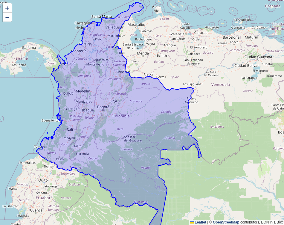
I ran the “Get Country Polygon” script, creating a nice Colombia polygon.
There is a drag and drop pipeline editor which felt a lot like Microsoft Access.
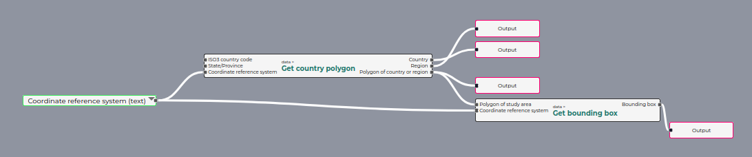
I followed along with the tutorial and created an R script and a YAML file of the same name in the /scripts directory. These appeared in the GUI, allowing me to run them and use them in the pipeline editor. Annoyingly, the dataset was not provided in the tutorial, so I couldn’t run the code.
TestScript.R
The biab functions are how the script interacts with the BON in a Box system.
library(rjson)
library(sf)
library(terra)
library(dplyr)
library(ggplot2)

input <- biab_inputs()

dat <- st_read(input$country_polygon)

if (nrow(dat)==0) {
        biab_error_stop("Country polygon does not exist")
}

dat.transformed <- st_transform(dat, crs=input$crs)

rasters <- terra::rast(c(input$rasters, crs=intput$crs))

country_vect <- vect(dat.transformed)

raster.cropped <- mask(rasters, country_vect)

raster_change <- rasters[[1]]-rasters[[2]]

raster_change_path <- file.path(outputFolder, "raster_change.tif")
writeRaster(raster_change, raster_change_path)

biab_output("raster_change", raster_change_path)

layer_means <- global(rasters.cropped, fun="mean", na.rm=TRUE)
layer_means$name <- names(rasters.cropped)

means_plot <- ggplot(layer_means, aes(x=name, y=mean)) + geom_point()

means_plot_path <- file.path(outputFolder, "means_plot.png")
ggsave(means_plot_path, means_plot)

biab_output("means_plot", means_plot_path)
TestScript.yaml
The inputs and outputs section defines the inputs and outputs, where the names must match the names in the script above. The environment is set up using conda. A specific version can be specified like this: r-terra=0.9-12
script: TestScript.R
name: Test script
description: Demo script
author:
  - name: ME
inputs:
  country_ploygon:
    label: Country Polygon
    description: Polygon of the country of interest
    type: application/geo+json
    example: null
  crs:
    label: Coordinate reference system
    description: Coordinate reference system
    type: text
    example: "EPSG:3857"
  rasters:
    label: Rasters
    description: Raster layers of variable of interest
    type: image/tiff;application=geotiff[]
    example: null
outputs:
  raster_change:
    label: Rasters
    description: Differences between raster values
    type: image/tiff;application=geotiff
  means_plot:
    label: Plot of raster means
    description: Plot of means of raster layers
    type: image/png
conda:
  channels:
    - conda-forge
    - r
  dependencies:
    - r-rjson
    - r-sf
    - r-dplyr
    - r-terra
    - r-ggplot2
The architecture appears to be designed as a single-server instance without built-in job queuing or concurrent execution limits.