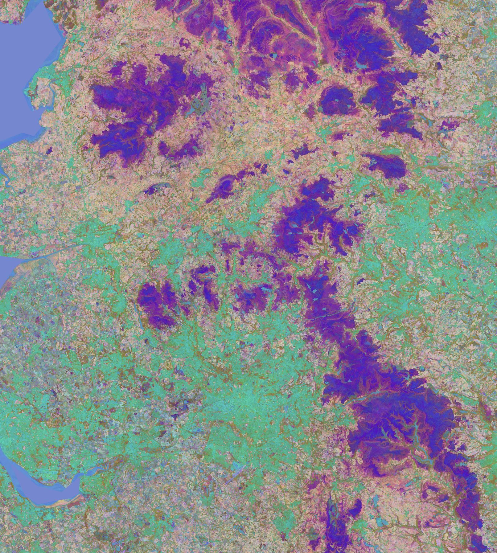
In my Intel AMX post I found that a few AMX cores could keep pace with a small GPU on the Tessera model. Since then, Intel has given us time on their Endeavour cluster, which is full of recent Xeons with no GPUs in sight. So I tried running the current model, the v2 pixel student, there.
Sadiq was surprised by how far CPU inference trailed the GPU and asked whether the gap was due to hardware or whether we were leaving performance on the table. Finding the missing performance took me from PyTorch to a standalone C++ program, and to be fair to the other side, I then gave the GPU the same treatment.
Everything below uses one test tile near Manchester, grid_-1.65_53.35, which is 1125 by 687 = 772,875 pixels for the year 2024. Every optimised version was checked against the published v2 embeddings for that tile.
The starting point #
The published code is PyTorch with bf16 autocast. It is the version that emerged from the development cycle rather than a built-for-speed version. On a dual-socket Xeon 6980P node, which has 2 x 128 cores, it managed this:
| Configuration | Result |
|---|---|
| 16 processes of 16 threads, whole node | 56 tiles per hour |
| One process, all 256 cores, threads not pinned | 1,782 s per tile |
| One process, all 256 cores, threads pinned | 194 s per tile |
The difference between the second and third row is astonishing: without pinning, the OpenMP threads wandered onto hyperthread siblings and between cores, and a single tile took half an hour. Pinning the same 256 threads to physical cores made it nine times faster. Nothing that follows is quite that dramatic, but it shows that very capable hardware can look bad when driven incorrectly.
Count the work first #
The model is two small transformers, one for Sentinel-2 and one for Sentinel-1, each with four layers of width 640 and a feed-forward width of 2,560, followed by a small fusion head. Every pixel is independent, and the work per pixel depends only on the number of observations it has, because the code pads each time series to the next multiple of 8.
def backbone_flops(T, bands, d=640, f=2560, layers=4):
  emb = 2 * T * (bands * d + d * d)
  per_layer = 8 * T * d * d + 4 * T * T * d + 4 * T * d * f
  return emb + layers * per_layer
Summing that over every pixel’s actual sequence lengths yields 4.56 PFLOP for the Manchester tile, and 97.5% of that is plain matrix multiplication. That means that the ceiling of this inference is how fast each machine can multiply bf16 matrices.
The cheap experiments #
Native bf16, instead of autocast, removes the casts that autocast inserts around every operation, which saved 7%. However, the model feeds the raw day-of-year into sine and cosine positional encodings, and bf16 has only 8 significant bits, so above 256 it can only represent even numbers. Every odd day after 256 rounds onto a neighbour. I kept that one input in float32:
bands = x[:, :, :-1].to(torch.bfloat16)
doy = x[:, :, -1].float()                 # exact day of year, never through bf16
h = self.embedding(bands) + self.temporal_encoder(doy).to(torch.bfloat16)
torch.compile was 7% slower with dynamic shapes. With static shapes, it was 14% faster on a test set, but every combination of sequence lengths needs its own compile, which makes it awkward to use.
OpenVINO was 38% slower out of the box, and less accurate.
None of this made a significant improvement, so I went looking for what the hardware ceiling actually was.
Measuring the hardware, not the framework #
Intel’s oneDNN ships a benchmark tool called benchdnn. I built it on the cluster and ran the model’s exact matrix shapes through it, alongside the same shapes run by PyTorch. Both use the same AMX kernel underneath, so I expected similar numbers, but I did not get them.
| 16 threads, 457k rows | PyTorch | benchdnn |
|---|---|---|
| Attention output, 640 to 640 | 12.4 TFLOPS | 24.2 TFLOPS |
| Feed forward up, 640 to 2560 | 12.5 TFLOPS | 26.6 TFLOPS |
| Feed forward down, 2560 to 640 | 10.9 TFLOPS | 18.1 TFLOPS |
oneDNN’s verbose log showed the reason: PyTorch hands the weights over in their plain row-major layout on every call, so the kernel reorganises them each time, whereas benchdnn lets oneDNN reorder them once into the blocked layout AMX wants. PyTorch exposes the ops it uses internally, so I could pack the weights myself:
packed = torch.ops.mkldnn._reorder_linear_weight(weight.to(torch.bfloat16), 4096 * 112)
y = torch.ops.mkldnn._linear_pointwise(x, packed, bias, "relu", [], "")             # ReLU fused
y = torch.ops.mkldnn._linear_pointwise.binary(x, residual, packed, bias, "add")     # residual fused
Rewriting the encoder layer around these calls, with the ReLU and the residual additions folded into the matrix multiplies, took the node from 56 to 82 tiles per hour.
Allocations that cost more than the maths #
The packed version was still slower per call than benchdnn. PyTorch allocates a fresh output tensor for every operation, and for the feed-forward layer, a batch of 4,096 pixels requires 2.2 GB. glibc serves anything over 32 MB with a new mmap, so every call page-faults and zeroes 2.2 GB before doing any useful work. A microbenchmark put that at 29% of the call.
You cannot raise glibc’s threshold past 32 MB, but you can tell it never to use mmap and never to give memory back, so big blocks are reused from the heap:
export MALLOC_MMAP_MAX_=0
export MALLOC_TRIM_THRESHOLD_=68719476736
export MALLOC_TOP_PAD_=1073741824
Three environment variables and no code changes took the node from 82 to 97 tiles per hour.
The clock drops when every core is busy #
At this point, I had a single 16-thread process which ran a single tile quickly, but it did not scale to the whole node. Running sixteen of them together should have given about 170 tiles per hour, not 97. Counting cycles with perf stat during the real inference showed the root cause.
| Processes running | Clock while running | Time per tile |
|---|---|---|
| 1 | 3.39 GHz | 380 s |
| 4 | 2.80 GHz | 489 s |
| 8, one socket full | 2.45 GHz | 533 s |
| 16, both sockets full | 2.47 GHz | 538 s |
The clock falls by 27% once a socket is full of AMX work, which accounts for about 95% of the slowdown. Memory bandwidth was not the problem: the node was using about a third of what STREAM showed it could deliver. Other chips on the cluster behave differently. The small 32-core-per-socket 6745P barely throttles, while the older Emerald Rapids and Sapphire Rapids parts sit right at their power limit and drop by about 30%.
Where the rest of the time went #
Factoring in the throttling, if every FLOP ran at oneDNN’s own full-load rate, the node should still manage about 160 tiles per hour, whereas I was at 97. Profiling the PyTorch path showed that about 85% of the difference was work other than matrix multiplication. Attention runs on tiny 112 by 112 matrices, one per pixel and head, which keeps AMX underfed. LayerNorm and the residual additions are pure memory traffic.
That second part is the interesting one. At a batch of 4,096 pixels, every intermediate tensor inside a layer is between 587 MB and 2.35 GB, and a 16-thread process has roughly 95 MB of cache. So every step writes its whole output to DRAM, and the next step reads it straight back.
Writing in blocks that fit #
Years ago, I saw a presentation from Nimble Storage showing how they got massive performance gains from spinning disks by noticing that sequential writes were fast. They organised their data into blocks that exactly matched the width of the disk array and wrote continuously. The same idea applies here: the data needs to be the right size. Instead of pushing all 4,096 pixels through one operation and then the next, take a small block of pixels through the whole layer while it is still in cache, then move on.
AMX does not need huge matrices to stay busy. One instruction multiplies a 16-by-32 tile by a 32-by-16 tile, so a block of 32 pixels, which is 3,584 rows, still requires hundreds of tile operations per matrix multiply. I wrote a C++ microbenchmark of one encoder layer against oneDNN, with the block size as the only variable.
The first results were confusing because my matrix-multiply runs were 1.6 to 2 times slower than benchdnn on identical shapes. The cause was buffer alignment. std::vector only guarantees 16-byte alignment, so every AMX tile load straddled two cache lines. Allocating on 2 MB boundaries fixed it:
p = std::aligned_alloc(2u << 20, bytes); // was: std::vector<uint16_t>
| One layer, one batch | One process, 16 threads | Whole node busy |
|---|---|---|
| Published PyTorch | 346 ms | about 490 ms |
| C++, whole batch, 16-byte aligned | 437 ms | 658 ms |
| C++, whole batch, 2 MB aligned | 296 ms | 493 ms |
| C++, blocks of 32 pixels | 269 ms | 392 ms |
With the node fully loaded, blocking was about 20% faster per layer than the published path, and every operation in the layer got cheaper.
The whole model in C++ #
The next step was the full forward pass in C++, including both backbones, attention pooling, and the fusion head, called from the existing Python batching via ctypes. The first full-tile run was a disaster at 26 tiles per hour.
The culprit was OMP_WAIT_POLICY=PASSIVE, carried over from the PyTorch job scripts. A block of 32 pixels runs about 80 oneDNN operations, and a tile has about 24,000 blocks, so there were nearly two million OpenMP parallel regions per tile. With the passive policy, each one had to wake 16 sleeping threads through the kernel. Switching to ACTIVE fixed most of it, but there was still a barrier at the end of every operation.
oneDNN can be built with a sequential runtime, where every call simply runs on the thread that made it. Each thread then takes its own block of a few pixels through the entire model, alone, and never waits for anyone:
#pragma omp parallel for schedule(dynamic, 1)
for (int64_t block = 0; block < nblocks; ++block) {
  Scratch &s = per_thread_scratch[omp_get_thread_num()];
  run_backbone(s, sentinel2, block);        // 4 layers, single-threaded oneDNN calls
  run_backbone(s, sentinel1, block);
  run_fusion_head(s, block);
}
Pixels are independent, so this needs no synchronisation at all. With 4 pixels per thread, the node reached 122 tiles per hour.
A per-phase profile then showed the matrix multiplies running at the same rate per core as benchdnn’s full-load figure, which is to say at the hardware ceiling. Two small things were still worth doing. Sentinel-2 series are shorter than Sentinel-1, so their matrix multiplies were thin, and giving S2 a larger block than S1 added 5%. I also made the process layout socket-aware so that no process straddles two sockets.
No Python at all #
The library still relied on Python to load the tile, bin each pixel by its number of observations, choose and pad the observations, standardise them and quantise the result. Moving all of that into C++ gave a single program:
tessera_encode TILE_DIR OUT_DIR student_large.tcw
The fiddly part was matching NumPy. The padding uses np.linspace(..., dtype=int64), which floors float64 values and pins the last element, and np.array_split, which gives the leftover elements to the first groups:
if (n >= B) {                                   // np.linspace(0, n-1, B) as int64
  const double step = double(n - 1) / double(B - 1);
  for (int64_t i = 0; i < B; ++i) out[i] = int64_t(std::floor(i * step));
  out[B - 1] = n - 1;
}
I tested it against the Python function on 2,400 cases with no mismatches, and on the full tile the C++ program writes output files that are byte-for-byte identical to the Python path. It is also faster because preparing each batch now takes milliseconds on the same threads, rather than seconds with single-threaded NumPy. The node went from 128 to 136.5 tiles per hour.
Giving each process its cores’ hyperthread siblings made it 25% slower, as both siblings share one AMX unit and one L1 and L2 cache, so a second thread just splits them and the blocks no longer fit.
Across the cluster #
Every chip type gained between 30% and 90% over its best PyTorch configuration.
| Chip | Cores | Tiles per hour | Best PyTorch | Eager PyTorch |
|---|---|---|---|---|
| Xeon 6980P | 2 x 128 | 128.3 | 96.6 | 56.2 |
| Xeon 6972P, MCR memory | 2 x 96 | 123.4 | 90.8 | 50.8 |
| Xeon 6972P, DDR memory | 2 x 96 | 122.7 | 86.6 | 46.9 |
| Xeon 6966P-C | 2 x 96 | 119.3 | 87.8 | 46.1 |
| Xeon 6787P | 2 x 86 | 85.7 | 45.2 | 30.0 |
| Xeon 6767P | 2 x 64 | 83.5 | 58.3 | 31.2 |
| Xeon 8592+, Emerald Rapids | 2 x 64 | 67.8 | 48.3 | 24.8 |
| Xeon 6745P | 2 x 32 | 57.6 | 36.9 | 19.6 |
| Xeon 8480+, Sapphire Rapids | 2 x 56 | 45.1 | 34.6 | 19.8 |
These use the C++ library called from Python. The standalone program adds about 6% on top, measured so far on the 6980P only.
On PyTorch, the 6972P with faster MCR memory was 8% faster than the same chip with ordinary DDR. With cache-sized blocks, the two are level, even though MCR has 24% more bandwidth. That is about as direct a demonstration as you can get that the blocks took main memory off the critical path.
I also timed a single tile with one process using every core to test how quickly you can produce a single tile. The AMD machine is monteverde, which featured in my GPU vs CPU post.
| Machine | Cores | Matrix unit | One tile |
|---|---|---|---|
| Xeon 6980P | 256 | AMX | 32 s |
| Xeon 6972P | 192 | AMX | 34 s |
| Xeon 8592+ | 128 | AMX | 50 s |
| AMD EPYC 9965 x 2 | 384 | AVX-512 bf16, no AMX | 67 s |
| Xeon 8480+ | 112 | AMX | 81 s |
Monteverde has 1.5 times the cores of the 6980P and takes twice as long, which puts AMX at about three times AVX-512 bf16 per core on this model.
Giving the GPU the same treatment #
It would not be fair to spend days tuning the CPU and then compare it with untuned GPU code, so I repeated the process on monteverde’s NVIDIA L4.
| L4, Manchester tile | Time per tile |
|---|---|
| Eager PyTorch, today’s published path | 227 s |
| torch.compile | 170 s |
| TensorRT | 166 s |
Getting TensorRT to work was awkward because the model builds its positional encoding by assigning into alternate columns, and TensorRT’s converter for that operation failed with dynamic shapes. Interleaving with stack instead gives the identical tensor and converts cleanly:
# original: pe[..., 0::2] = sin(a); pe[..., 1::2] = cos(a)
pe = torch.stack([torch.sin(a), torch.cos(a)], dim=-1).flatten(-2)
As with the CPU, I measured the hardware ceiling. A cuBLASLt benchmark on the model’s shapes showed the same effect as on the Xeons: small chunks that fit in the L4’s 50 MB of L2 cache ran about 40% faster than full batches. The L4 has a 72 W power budget, and under sustained matrix work its clock fell to a median of 945 MHz, less than half its 2,040 MHz maximum. At that clock, cuBLASLt was already at its limit, which puts the best possible time for this tile at about 83 s.
Because the C++ encoder talks to its network through four functions, the GPU version did not need a new program. I wrote a CUDA library with the same interface and linked the unchanged encoder against it:
void *tc_create(const char *weights, int block);
int   tc_encode(void *h, const float *s2, int64_t G, int64_t T2,
              const float *s1, int64_t T1, float *out);
void  tc_profile_dump(void *h);
void  tc_destroy(void *h);
Each chunk of 64 pixels runs both backbones and the fusion head before the next chunk starts. The matrix multiplies use cuBLASLt with the bias, ReLU and residual folded into the same call, with the residual going in as beta * C. LayerNorm, input preparation and attention pooling are small custom kernels.
| L4, Manchester tile | Time per tile | Speed-up over eager |
|---|---|---|
| Eager PyTorch | 227 s | 1.0 |
| TensorRT | 166 s | 1.4 |
| C++ and CUDA, chunked | 117 s | 1.9 |
| Ceiling at the L4’s power-limited clock | about 83 s | 2.7 |
Chunk size matters for the same reason block size did on the CPU. Above 64 pixels, the chunk’s intermediates outgrow the 50 MB L2:
| Chunk | 32 px | 64 px | 128 px | 256 px |
|---|---|---|---|---|
| Time per tile | 121 s | 117 s | 121 s | 127 s |
Two ideas did not pay off. CUDA Graphs cut the host’s launch work from 8.5 s to 0.8 s on a test crop, but the GPU time did not move because the GPU had never been waiting for launches. A fused attention kernel on the tensor cores came out no faster than three separate steps, because its shared-memory needs left room for only four warps per SM. A FlashAttention-style kernel that keeps the scores in registers might save another 15%.
How does that compare with dClimate’s engine? #
dClimate run Tessera in production with their own inference engine, and they have tuned it carefully for the GPUs they use: bucketing pixels by observation count, a batch of 7,168 in bf16, a pinned two-deep pipeline between host and GPU, and int8 quantisation on the device. To see where the C++ version sits against something already optimised, I drove the engine’s three per-strip calls directly, with no Ray, Zarr, S3 or Prefect around them:
model = build_inference_model(config, device, ckpt)
dataset = MosaicChunkInferenceDataset(ChunkData(...))   # bucketing and deterministic resampling
run_inference(model, dataset, config, device)            # pinned, pipelined GPU loop
Their band order and S1 encoding match my DPixel layout, so the arrays go in unchanged. On the same L4 and the same tile:
| Engine, v2 Large | Time per tile |
|---|---|
| C++ and CUDA, 64-pixel chunks | 117.0 s |
| dClimate, pipelined loop | 129 to 130 s |
| dClimate, serial loop | 130 to 132 s |
| dClimate, v1.1 model for comparison | 173 to 176 s |
All three v2 outputs agree with each other and with the CPU reference to the same bf16 envelope: about 92 to 94% of int8 values identical, at most 3 apart, cosine similarity 0.99997.
So the hand-written version is about 10% faster than an engine that was already carefully tuned, which is a smaller gap than the one between it and eager PyTorch, and that seems right. The engine runs the model through torch.compile, so it gets much of the fusion for free, and what it cannot do is keep a chunk’s whole forward pass resident in L2.
Their pipelined loop, which overlaps host preparation with GPU work, bought under 1% here. On a power-capped L4 the forward pass is so much slower than the CPU preparation that the host never holds the card back. The card sat at its 72 W cap for the entire run with the SM clock between 780 and 1,080 MHz.
So how big is the gap? #
With both sides optimised, one 6980P node completes a tile in 32 s and the L4 does it in 117 s. A single Xeon node is worth almost four of these cards, and monteverde’s own AMD CPUs beat its GPU. That probably says more about the L4 than about GPUs in general: it is a 72 W inference card that spends most of its time at less than half its rated clock.
The larger GPU this project originally ran on, an MI355X, I no longer have access to, so I cannot measure the Manchester tile on it. Scaling a single earlier timing by FLOP count suggests roughly 24 s per tile, or about 150 tiles per hour per GPU. On that estimate, one Xeon node is within about 10% of one MI355X, though an eight-GPU node is still close to an order of magnitude ahead. That GPU was also only using about 8% of its peak, so it has headroom of its own, and the L4 work shows how to start recovering it.
Scorecard #
The final scorecard on the 6980P node:
| Step | Tiles per hour | Gain over eager |
|---|---|---|
| Eager PyTorch | 56.2 | 1.0 |
| Packed weights, fused ReLU and residual | 81.9 | 1.5 |
| Plus heap-only malloc | 96.6 | 1.7 |
| C++, thread per block | 122.3 | 2.2 |
| Plus a separate S2 block size | 128.3 | 2.3 |
| Standalone C++ encoder | 136.5 | 2.4 |
The code #
The final encoder is at mtelvers/tessera-inference. It is a single C++ program, tessera_encode, which reads a staged tile and writes the int8 embeddings and scales. You can build it against oneDNN for the CPU or against cuBLASLt for an NVIDIA GPU. A small Python script converts the published v2 checkpoint into the flat weights file the encoder reads, and the README covers building oneDNN with the sequential runtime and the settings that matter.