Mandelbrot Set 3D

Back in 2015 in one of the earliest posts on this site I wrote about my fascination with the Mandelbrot set.

\[Z_{n+1}=Z_n^2+c\]

In that post, I presented a table of giving two example iterations with different values of C showing both a bound and unbound condition. I’d never really thought about the actual value the bound series tended towards, after all the final plot was the number of iterations it took to become unbound. i.e. where \(\lvert Z \rvert > 2\)

Watching an episode of Numberphile on YouTube, it became clear that I’d really missed out on some interesting behaviour… about rabbits, which then led me to a second video and a view of the Mandelbrot set as I’d never seen it before.

The table below mirrors that I presented my by original post but additionally shows the outcome at \(C=-1.3\).

	C = 0.2	C = 0.3	C = -1.3
0	0.000000	0.000000	0.000000
1	0.200000	0.300000	-1.300000
2	0.240000	0.390000	0.390000
3	0.257600	0.452100	-1.147900
4	0.266358	0.504394	0.017674
5	0.270946	0.554414	-1.299688
6	0.273412	0.607375	0.389188
7	0.274754	0.668904	-1.148533
8	0.275490	0.747432	0.019128
9	0.275895	0.858655	-1.299634
10	0.276118	1.037289	0.389049
11	0.276241	1.375968	-1.148641
12	0.276309	2.193288	0.019376
13	0.276347	5.110511	-1.299625
14	0.276368	26.417318	0.389024
15	0.276379	698.174702	-1.148660
16	0.276385	#NUM!	0.019421
17	0.276389	#NUM!	-1.299623
18	0.276391	#NUM!	0.389020
19	0.276392	#NUM!	-1.148664
20	0.276392	#NUM!	0.019429
21	0.276393	#NUM!	-1.299623
22	0.276393	#NUM!	0.389019
23	0.276393	#NUM!	-1.148664
24	0.276393	#NUM!	0.019430
25	0.276393	#NUM!	-1.299622
26	0.276393	#NUM!	0.389019
27	0.276393	#NUM!	-1.148665
28	0.276393	#NUM!	0.019430
29	0.276393	#NUM!	-1.299622
30	0.276393	#NUM!	0.389019
31	0.276393	#NUM!	-1.148665

At \(C=-1.3\) there is a clear repeating pattern of four values.

In Excel set row 1 as the value of C starting at -2 and incrementing by say 0.02 up to 0.0. Then run the iterations in columns below each value starting at 0. Extend the columns for perhaps 40 iterations.

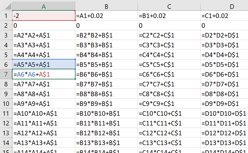
Now plot iterations 20-40 (when the values are typically stable) against the value of C.

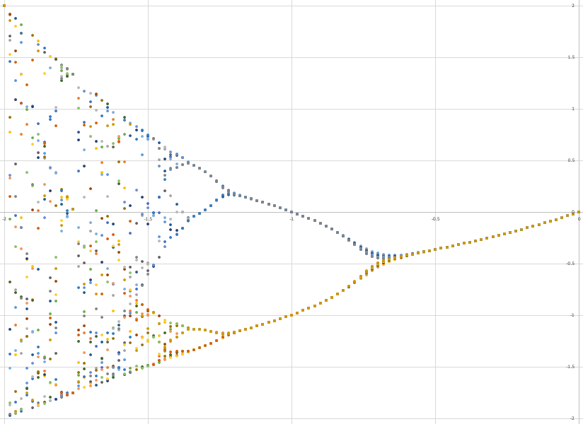
I want to plot the real component of C on the x-axis, then imaginary component on the y-axis and the real part of the iterated sequence on the z-axis. Where the sequence repeats I’ll plot all points within the sequence which looks to be what was done in the YouTube clip.

I’m sitting here with my new, albeit secondhand, Mac Pro so let’s write this in Swift and do all the calculation and graphics on the GPU using Metal.

The problem is well suited to GPU based calculations with a small kernel running once for each possible set of input coordinates, however the output of a massive sparsely populated three dimensional array seemed unfortunate. Suggesting a resolution of 2048 x 2048 and allowing iterative sequences of up to 1024 gives potentially 4 billion points… Therefore, I have opted for an output vector/array indexed with a shared atomically-incremental counter.

To use the GPU to perform the calculations the program needs to be written in Metal Shading Language which is a variation on C++, but first the GPU need to be initialised from Swift which for this project is pretty straightforward. We’ll need a buffer for the output vector and another one for the counter:

vertexBuffer = device.makeBuffer(length: MemoryLayout<Vertex>.stride * 2048 * 2048, options: [])
counterBuffer = device.makeBuffer(length: MemoryLayout<UInt>.size, options: [])

Then we create a library within the GPU device where the name parameter exactly matches the MTL function name we want to call

let library = device.makeDefaultLibrary()
let calculate_func = library?.makeFunction(name: "calculate_func")
pipeLineState = try device.makeComputePipelineState(function: calculate_func!)

The calculate_func is defined as follows

kernel void calculate_func(device VertexIn* result,
                            uint2 index [[ thread_position_in_grid ]],
                            device atomic_uint &counter [[ buffer(1) ]]) {

    float bufRe[1024];
    float bufIm[1024];

    float Cre = (float(index.x) * 3 / 2048) - 2;
    float Cim = (float(index.y) * 3 / 2048) - 1.5;

    float Zre = 0;
    float Zim = 0;
    
    bufRe[0] = 0;
    bufIm[0] = 0;

    for (int iteration = 1; (iteration < 1024) && ((Zre * Zre + Zim * Zim) <= 4); iteration++) {
        float ZNre = Zre * Zre - Zim * Zim + Cre;
        Zim = 2 * Zre * Zim + Cim;
        Zre = ZNre;
                
        bufRe[iteration] = Zre;
        bufIm[iteration] = Zim;
        
        for (int i = iteration - 1; i; i--) {
            if ((bufRe[iteration] == bufRe[i]) && (bufIm[iteration] == bufIm[i])) {
                for (; i < iteration; i++) {
                    float red = abs(bufIm[i]) * 5;
                    float green = abs(bufRe[i]) / 2;
                    float blue = 0.75;
                    
                    uint value = atomic_fetch_add_explicit(&counter, 1, memory_order_relaxed);
                    result[value].position = float3(Cre, Cim, bufRe[i]);
                    result[value].color = float4(red, green, blue, 1);
                }
                return;
            }
        }
    }
}

The first section is the standard calculation for \(Z_{n+1}\). The nested loop searches back through the previous values to see if we have had this value before. While this should be an exhaustive check of every value, I haven’t done that for performance reasons, but I did leave the check to be the exact floating point value rather than just 2 or 3 decimal places. If there is a match then all the points are copied to the output vector in a pretty colour.

You can see the full code on Github.

Categories